A messy roommate who doesn’t cleanup after guests. A significant other who doesn’t take out the trash. A sibling that clutters the bathroom counter. We’ve all encountered (or will encounter) one of these people in our lives: those that unknowningly or otherwise take advantage of shared communal resources. Can these types’ menacing behaviors be explained by rational methods or will their ways forever evade the good Samaritans of the household? In this blog series, we will use economic analysis to shed light on the incentives of cooperation and selfishness and perhaps learn something about ourselves and others in the process. Later in the series, we will breach out from the household and analyze cooperation and selfishness on a global scale: pollution, climate change, and various other issues involving communal resources.
In this article, we’ll cover various economic concepts such as:
- Utility functions
- Opportunity Cost
- Game Theory
We’ll begin with a few core concepts of economics and continue on to the rest of the article.
Beware, this is an article that features math, the (especially) boring details are hidden behind dropdowns where the interested reader can dive deeper if they so choose.
Core Concepts
Utility
The single core concept of the study of economics is utility. You can think of utility as happiness. The more utility the better. It is assumed to be the one thing economic agents strive to maximize. Economists’ notion of utility is roughly modelled to account for real-life facts: that as you consume or do one particular thing, your increase in utility decreases. Every cookie after the first brings less happiness and may even make you unhappy.
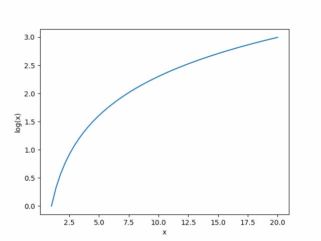
A very common utility function is the logarithm function (log for short):

which we can see seems to level off as gets large. Many other functions will work but the mathematical ease-of-use of the log function makes it a very popular choice.
Opportunity Cost
The next core concept of economics is opportunity cost which stems from the idea of limited resources. Choosing to use your farm for apples means that you cannot also use it for wheat. You can eat an apple or an orange but you’ll only have so much space in your stomach. We can augment our utility function to take account of this concept:
subject to
Let’s say is for apples and is for oranges. So we can see that consuming either apples or oranges gives us utility, however, notice the new constraint: we can only eat an amount of either apples or oranges.
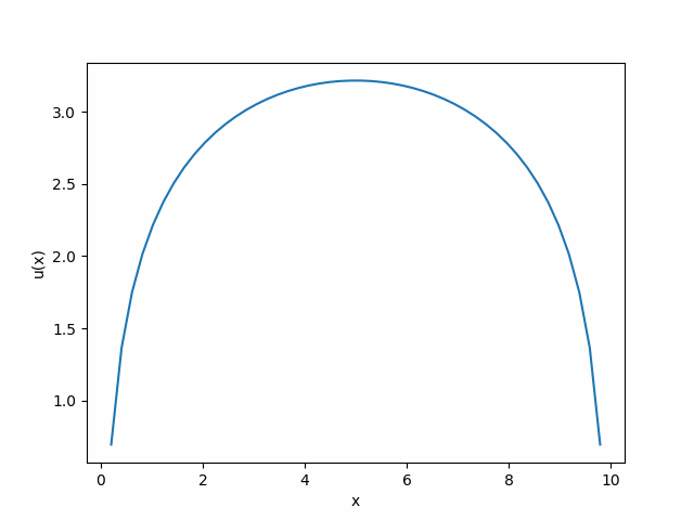
For example, say we can only eat 10 apples or oranges and let’s use the new constraint to simplify our utility function to be a function of only the number of apples we eat.

Due to the symmetry of our utility function, we can clearly see it is maximized when we eat 5 apples and 5 oranges.
Preferences
What happens if we like apples slightly more than oranges? We can add multipliers to the components of our utility function:
is how many times more we like apples over oranges and vice versa.
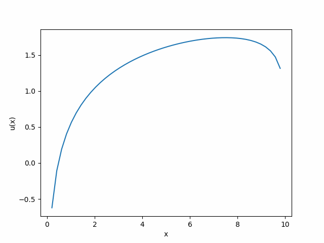
For example, say and . That means I like apples 3 times more than oranges. Taking into account opportunity cost like above and assuming I can only eat 10 apples or oranges our utility function now looks like:

which is maximized when I eat 7.5 apples and 2.5 oranges. If I like apples 3 times more than oranges, I will eat 3 times as many.
-
To optimize for utility with respect to the inputs, economists are concerned with finding the points of indifference. That is, the allocation of the inputs such that no one component has an “edge” over the other.
If you know calculus, this might sound oddly like a derivative (aka sensitivity to change) where we are concerned with finding the 0’s of a derivate (aka a critical point).
I like to think of practical interpretations of this mathematical concept: you will consume items or engage in various activities but generally will spread out your time and money so that each component of your utility is given as much input as the effect on your total output (utility) is called for.
A Simple Household
Now the fun part, let’s consider Alice and Bob, two young adults living together splitting chores. Let’s construct utility functions for both of them by considering two activities that either of them can engage in: chores or leisure. However, there is a twist: the chores are communal meaning Bob will still gain utility from a clean house even if Alice does the chores.
Let’s say is the time spent on doing chores, for time spent on leisure, in general subscripting Alice’s variables with , Bob’s variables with , and the sum of Alice and Bob’s variables with when there could be ambiguity.
Then the utility function for Alice would be
Assuming that both of them have 100 hours to spend between leisure or chores, let’s rewrite this as
Cooperative Utopia
Let’s say Bob has preferences and (preferring leisure) and Alice has preferences and (evenly split).
Using similar logic to the first section of this article, we can solve for the time allocation that maximizes total household utility (the sum of both their utilities ):
-
We can reduce this problem by combining Alice and Bob’s time so that
and solving
gives that .
Now, looking at the combined utility again using we get
which is a utility function of one variable which we solved in a section above.
(We can combine the utility functions and talk about this new one as written here due to the nice properties of the log function as mentioned but this general result will hold via traditional optimization which we go over in a later section.)
which turns out to be and .
Bob spending 25 hours on chores and 75 hours on leisure; Alice spending 50 hours on chores and 50 hours on leisure. Everyone happy.
Bob the Slob
However, there’s a problem with our utopia (shocker).
Let’s take a closer look at Bob’s utility function
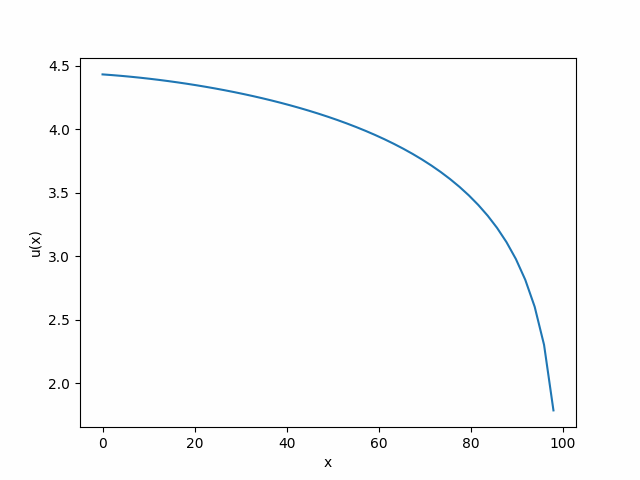
Assuming Alice does the optimal amount of 50 hours of chores, Bob’s utility function becomes

which is maximized when Bob does 0 hours of chores. Less than if he lived alone!
This is because Alice is already doing 50 hours of chores: more than what Bob “prefers” should be done. This outcome is “stable” as well: knowing Bob’s time allocation, Alice should still do 50 hours of chores to maximize her own personal utility while Bob spends all his time on leisure.
So what’s happening?
Game Theory
Game theory is the study of economic agents whose utility functions not only depend on their own actions but other agents’ actions as well, much like how Alice and Bob’s optimal time allocations depend on each other. We’ll have another article that examples game theory in depth, but we’ll cover the basics now to handle this chore dispute with Alice and Bob.
At the heart of game theory is Pareto efficient outcomes, which are outcomes like Alice and Bob’s above where the agents do not wish to switch their actions even knowing the other one’s choice. Let’s take a look at two little-known firms Coca-Cola and Pepsi for an example.
Coca-Cola & Pepsi
A very common technique of game theory is to draw a table to find the Pareto efficient outcomes. Let’s say Coca-Cola and Pepsi want to advertise their drink products.
- If neither of them advertise, consumers will continue to buy their preferred brand.
- If only one of them advertises, they will be dominate the market as consumers have one brand on their mind.
- However, if both of them advertise, consumers are back to square one, except this time both brands have to pay for their expensive marketing campaigns.
We can capture these scenarios in a payout table.
Let’s say Coca-Cola is the column-player, Pepsi is the row-player. Each cell is formatted as <column player reward> / <row player reward>.
| Don’t Advertise | Advertise | |
|---|---|---|
| Don’t Advertise | 500 / 450 | 250 / 650 |
| Advertise | 750 / 150 | 475 / 425 |
Let’s put ourselves in Coca-Cola’s shoes to decide as a business what should be done.
- If Pepsi doesn’t Advertise (first column), then 500 vs 750 means that we should Advertise.
- If Pepsi Advertises (second column), then 250 vs 475 means that we should Advertise.
So, Coca-Cola should Advertise regardless of action by Pepsi and vice versa!
The Pareto efficient outcome in this scenario is that both companies advertise, even though they both could make more money if they both didn’t advertise.
Fascinating enough, companies in real life faced with similar game theory problems agree to cooperate with each other to achieve outcomes that increase both parties’ profits. (This is oftentimes heavily regulated as this is potentially illegal collusion which hurts consumers.)
Alice & Bob
Let’s see if we can apply what we learned to Alice and Bob.
Notice that Bob’s utility function in the last section depends on Alice’s time allocation. In fact, given Alice’s time allocation, we can figure out exactly how much time Bob should allocate to chores to maximize his utility (and vice versa).
-
To find the optimal time allocation, we will find the solution of indifference. That is, the allocation that Bob will be equally happy spending the next hour on leisure or chores.
Recall Bob’s utility function
We set the derivative (aka sensitivity to change) equal to 0 to find the point of indifference.
Then, plugging in
It’s possible for Alice to be spiteful and spend all her time on leisure, forcing Bob to spend 25 hours on chores. (However, this would not maximize Alice’s utility. In general, economists assume that economic agents are rational, always trying to maximize their personal utility. There is a whole field of economics that studies irrational agents and its implications.)
So knowing that Alice’s optimal time allocation depends on his own time allocation, Bob can solve for the Pareto efficient outcome:
-
Using the conditional optimal time allocations from above
We can plug one in to the other
Then, plugging in
However, time has to be positive, so
Plugging this in to Alice’s equation we get
which we saw before resulted in
Bob does 0 hours of chores and Alice does 50 hours of chores.
Conclusion
In this article, we covered core concepts of economics including utility and opportunity cost, and touched on a little game theory. We applied these concepts to study a simple household that splits chores and learned something disconcerting: that the “lazy bums” we encounter in our lives are actually clever geniuses of game theory and are optimally maximizing their own personal utility (at the expense of the aggregate utility).
However, do not fret for real life examples show us that cooperation (such as in the case of companies’ non-compete agreements) is possible and even necessary in scenarios such as our simple household. In the next part of this series, we will investigate possible remedies to Alice and Bob’s utility functions so that even Bob the Slob with his resentment of chores will find it optimal to help out!